Introduction
In previous tutorials like this one, we have created a few projects using neural network models. However, if we want to train custom neural network models from the scratch, we need to use computers that are much more powerful (and expensive) than a Raspberry Pi. Fortunately, neural network is not the only way that we can implement machine learning. Raspberry Pi can run some machine learning algorithms really well, so we can do some ML experiments with it.
In this tutorial, we will:
- look at the basic concept of decision tree,
- load a dataset from a csv file with pandas,
- split the dataset for training and evaluating a model,
- create, use and evalutate a decision tree model with scikit-learn.
What is a Decision Tree?
We often need to make a decision based on different conditions. Consider the following decision making process for a weekend activity:
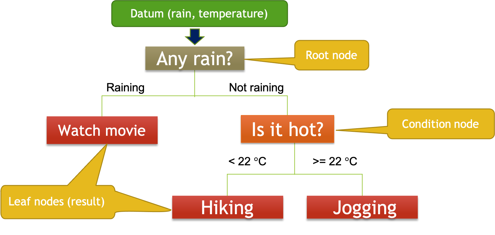
Suppose we only make the decision based on whether it’s raining and the temperature. We start with the first question (is it raining?) and split the decision tree into two branches (raining and not raining). If it’s raining, we will watch a movie. If it’s not raining, we split that branch further by considering the temperature. If it’s lower than 22 degree, we go hiking. Otherwise, we go jogging. From now on, we can make our decision by checking whether it’s raining and the current temperature, and use the decision tree to produce the result.
The next logical problem is how we can generate such a decision tree. This is where machine learning can help. Specifically, supervised learning can be used to generate a decision tree. In supervised learning, labelled data are put into learning algorithms to generate the rules (or ‘train the models’) that can be used for making predictions. If you want to know more about the concept of supervised learning, you should definitely check out this video from Google’s TensorFlow.
If we have lots of data in the format of (rain, temperature, activity), we can deduce the rules by looking at the pattern of the data. It turns out we can produce a decision tree by partitioning the predictors rain and temperature. The actual algorithm of generating a decision tree is out of the scope of this tutorial. If you want to know more details about decision trees, you should check out Chapter 8 of Introduction to Statistical Learning with Application of R.
Prerequisites
In this tutorial, we will use Visual Studio Code and Jupyter to do the hands-on task. You should follow this tutorial to setup Visual Studio Code and Jupyter on the Raspberry Pi if you have not done so.
Download and Open the Jupyter Notebook
If you’ve done all the setup, visit this repository and download it as a zip file.
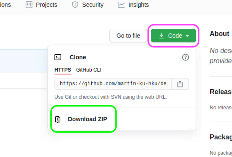
After the download is completed, right click the zip file and select Extract Here to unzip it. Right click the extracted folder and select Visual Studio Code to open the folder in Visual Studio Code.

In the sidebar, double click the Jupyter notebook to open it.
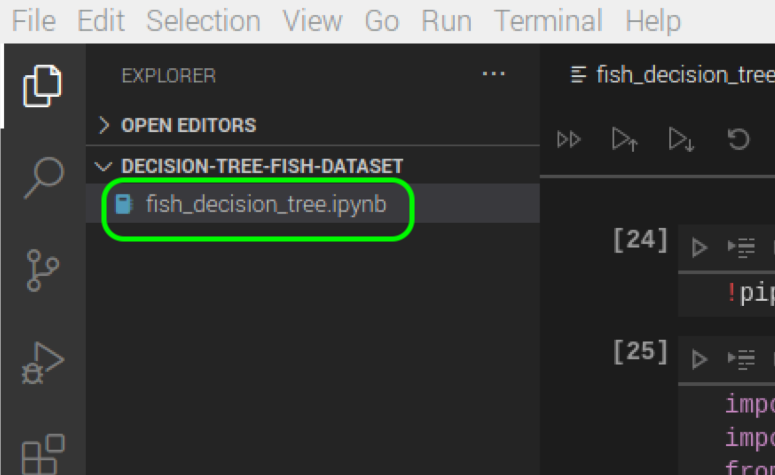
NOTE: If you receive a warning when opening the notebook, simply click ‘Trust’ to dismiss the warning.
Feel free to modify the notebook and do experiments with it. You may use the print function to print out the variables whenever necessary.
Download the Data
In this tutorial, we will use this fish market dataset from Kaggle. It’s a very small dataset that records 7 common different fish species in fish market sales. You can register a free account and download the data file. Once the file is downloaded, put the extracted csv file in the same folder as the Jupyter notebook. You can double click this csv file in the sidebar of Visual Studio Code and take a look of the data.
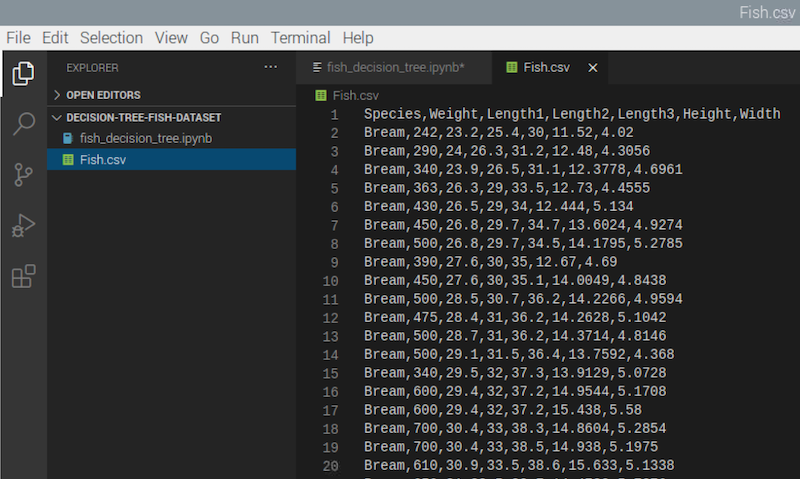
As you can see, each datum contains the name, the weight and different length measurements of the fish. You may check out the meaning of these measurements in this Kaggle discussion thread.
Install and Import the Libraries
Let’s go back to the Jupyter notebook. First, we need to install or update the necessary libraries. Execute the code in the first cell:
!pip3 install -U pandas sklearn graphviz
!sudo apt-get install graphviz -y
Then, we import the libraries that we need to use.
import pandas as pd
from sklearn.preprocessing import LabelEncoder
from sklearn.model_selection import train_test_split
from sklearn.tree import DecisionTreeClassifier, export_graphviz
from sklearn.metrics import accuracy_score
from IPython.display import display
import graphviz
pandas helps us load the data from the csv file into numpy arrays. sklearn helps us do almost all the machine learning tasks: precoess and split the data, as well as create, fit and evaluate the model. Finally, IPython.display and graphviz enable us to show the decision tree right inside the Jupyter notebook.
Load, Preprocess and Split the Data
Next, we can load the data from the csv file by the read_csv function of pandas library.
data = pd.read_csv('Fish.csv')
We can print out the first few data by calling the head function to make sure that the data file is loaded properly.
data.head()
Currently, data holds both the labels (the Species column) and the predictors (other columns). We need to separate them first.
X = data[['Weight', 'Length1', 'Length2', 'Length3', 'Height', 'Width']]
y = data['Species']
We will need the set of feature names when constructing the decision tree. We can get all the names of the columns by using the columns property of the pandas dataframe, and remove the first entry ‘Species’ by slicing the numpy array.
feature_names = list(data.columns[1:])
NOTE: If you want to know more about slicing numpy arrays, you may read this w3schools tutorial as a reference.
Machine learning algorithms work with numbers rather than texts. However, the y array contains the species names. Therefore, we need to encode them into numbers first. Scikit-learn provides a convenient way to do it. We can use the LabelEncoder class to encode the species names into numbers.
le = LabelEncoder()
le.fit(y)
class_names = list(le.classes_)
y = le.transform(y)
The fit function takes all the species names, and assign a number to each species. The classes_ property enables us to get all the names that have been encoded. Finally, we call the transform function to transform each of the entries of y from a string to a number.
When training a machine learning model, it’s often a good idea to withhold a portion of data, and use the withheld data for evaluating the model once the training is completed. Again, scikit-learn provides a convenient method for splitting the data into the training set and the testing set.
X_train, X_test, y_train, y_test = train_test_split(X, y, test_size=0.2, random_state=42)
Create and Train the Model
Creating and training the model is actually extremely easy. All we need to do is to create a DecisionTreeClassifier object, and call its fit function with the training data to train the model.
tree_clf = DecisionTreeClassifier(max_depth=4)
tree_clf.fit(X, y)
The max-depth argument sets the maximum height of the decision tree. In general, if the decision tree is taller, it can have a higher training accuracy, which means it can fit the training data better. However, a tall decision tree can lead to overfitting. Normally, the suitable height should be found by cross-validation. For our purpose, we just set that arbitrarily to 4. You may try using other values.
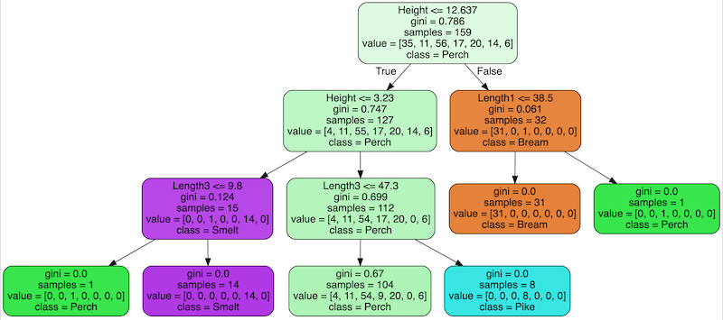
One of the great things about decision tree is that we can produce a graph that we can interrept very easily. To generate the graph of the decision tree, we can use the export_graphviz function.
display(graphviz.Source(export_graphviz(tree_clf, feature_names=feature_names, class_names=class_names, filled=True, rounded=True)))
NOTE: If you don’t supply the parameters
features_namesandclass_names, the graph will show the encoded numbers only.
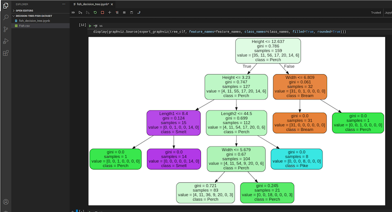
In each node, other than the name of the class, it also shows a number called ‘gini’. Basically it’s a number indicating how much ‘impurity’ is in that particular partition. When the tree splits further, the ‘gini’ should decrease down the way if the model fits well.
Make Prediction and Evaluate the Model
Making predictions is straightforward. We can do it with the predict function of the decision tree. Let’s make the prediction with the testing data.
y_pred = tree_clf.predict(X_test)
print(y_pred)
As you can see, the tree can make multiple predictions at the same time. We only need to pass the entire array of predictor data to the predict function.
Also, we can compare the predicted results with the true results of the testing data.
accuracy_score(y_test, y_pred)
The model has around 78% percent accuracy with the test data, which is not too bad for a simple model like this. We will discuss some methods to improve the accuracy in the future.
Conclusion
Machine learning sounds intimidating and complicated. However, as you can see in this tutorial, scikit-learn can make some machine learning tasks extremely simple. You may find other datasets from Kaggle and try making your own machine learning models. If you have any problem, you may ask us on our Facebook page.