Content
- Prologue
- Machine Learning
- Vector
- Represent information with vectors
- Affine transformation
- Deep neural network
- Train the neural network
- Summary
Prologue
Deep learning ignites the AI revolution in the past 10 years. We can often hear the news about ground-breaking technologies based on deep learning. You may wonder: since it’s so revolutionary and important, it must be something complicated? Well, not at all.
The idea of deep learning is actually incredibly simple. Moreover, it’s very easy to build your own deep learning models to solve your problems. You don’t need a degree in computer science, mathematics or statistics to become a deep learning expert. If you master a few fundamental concepts of deep learning well, and practice enough on framing and solving problems with deep learning, you can be a deep learning expert as well.
In this tutorial, we will attempt to solve this problem:
Given 4 different measurements of a flower, classify the flower into one of the three kinds of iris.
This problem may not look like a maths and coding problem at first, but we will frame this problem into one that is. Then, we will gradually construct our deep learning model when discussing and connecting different concepts of deep learning, and eventually solve this problem with our deep learning model. Let’s get started!
Machine Learning
First of all, we need to clarify three terms that are commonly used together: AI, machine learning and deep learning. The diagram below shows their relationships:
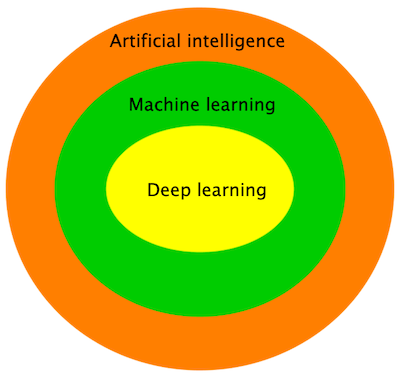
As we can see, machine learning is a kind of artificial intelligence (AI), and deep learning is a kind of machine learning. We will mainly discuss about deep learning in this tutorial, but let’s look at AI and machine learning first.
AI
AI are technologies that automate intellectual tasks performed by humans. Strong AI technologies, which can perform a wide variety of cognitive tasks like humans, currently only exist in fictions and movies. Weak AI technologies that can do specific tasks better than humans are the AI that we have developed so far.
Machine learning
In traditional programming, we define some rules and a computer program follow these rules to output the answers.

In machine learning, we input some data and answers to a program, and the program figures out the rules for us.

Supervised learning
Data together with answers are labelled data, and machine learning with labelled data is called supervised learning. In fact, there are unsupervised machine learning methods, but they are out of the scope of this tutorial.
A machine learning model is trained rather than pre-programmed. During the training, the model is presented with many examples. The training algorithms find the statistical structure of these examples. Once trained, the model can be used to make inferences.
Enough terminologies for now. Let’s look at a simple example of machine learning: finding a best-fit line. The following Python code generates some random data with linear relation and the best-fit line for the data.
import numpy as np
import matplotlib.pyplot as plt

xs = np.linspace(0, 10, 10)
deltas = np.random.randn(10)
ys = xs * 1.2 + deltas
m, c = np.polyfit(xs, ys, 1)
plt.scatter(xs, ys)
plt.plot(xs, m*xs+c)
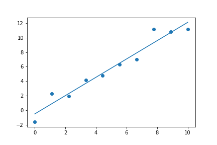
The following are the components of machine learning when finding the best-fit line:
- The dots in the scatter diagram are the data use for training the model. They have the inputs (x values) and the answers (y values).
- The learning algorithm (implemented by the
polyfitfunction) finds the statistical structure of the data (a straight line with particular slope and y-intercept). - After obtaining the best-fit line, we can use it to predict the y value for a given x value, i.e. to make inferences.
In short, machine learning is finding a function such that the function can turn the input into the answer we want.
After knowing what machine learning is, we can start learning about deep learning.
Vector
The first important concept of deep learning is vector, which is just an array of numbers. These are two examples of vectors:
\[\textbf{a} = \begin{pmatrix} 1\\ 2 \end{pmatrix} \text{, } \textbf{b} = \begin{pmatrix} 0.2\\ 0.4\\ -0.5\\ -0.8 \end{pmatrix}\]The number of entries in a vector is called the dimension. In the above examples, the dimension of \(\textbf{a}\) is 2, and the dimension of \(\textbf{b}\) is 4.
Dimension
This definition of dimension is for the context of deep learning only. In linear algebra, the term dimension describes the vector space rather than the vector itself.
In Python, we can use either a NumPy array to represent a vector. The vectors \(\textbf{a}\) and \(\textbf{b}\) in our examples can be created as follows.
NumPy
NumPy is a Python library that supports efficient operations on multi-dimensional arrays and matrices.
import numpy as np

a = np.array([1, 2])
b = np.array([0.2, 0.4, -0.5, -0.8])
Although vectors look simple, we will see that representing information with vectors (or vectorization) is an incredibly powerful tool to solve problems way beyond pure mathematics.
Represent information with vectors
The Iris flower data set is a classic data set for studying statistical learning. The data set contains 3 classes of iris plants (setosa, versicolor and virginica) of 50 instances each. Each instance contains the sepal and petal measurements. For example, the following is one of the instances in the data set.
- sepal length:
5.1 cm - sepal width:
3.5 cm - petal length:
1.4 cm - petal width:
0.2 cm - species:
setosa
We can easily represent the flower’s measurements with a vector.
\[\text{sizes} = \begin{pmatrix} 5.1\\ 3.5\\ 1.4\\ 0.2 \end{pmatrix}\]In fact, we can get a vectorized version of the Iris dataset from the sklearn Python package.
Sci-kit learn
Scikit-learn is a machine learning library that can be used for many kinds of machine learning tasks. It also comes with many data sets.
from sklearn import datasets
iris_dataset = datasets.load_iris()
features = iris_dataset['data']
print(features[:5]) # Show the first 5 data
The iris_dataset is a dictionary. The data entry is a NumPy array that contains the four features of all the data in the data set. As we can see in the first 5 data, these features are vectors already.
One-hot encoding
What about the species label, which is a categorical value? Let’s take a look of the target entry of iris_dataset.
labels = iris_dataset['target']
class_names = iris_dataset['target_names']
for label in labels[:5]: # print the first 5 targets
  print(f'target: {label} ')
  print(f'target in text: {class_names[label]}')
The class of flower in each datum is encoded with a number. 0 means setosa, 1 means versicolor, and 2 means virginica. We will use one hot encoding to turn it into a vector. Since the data set contains 3 classes of iris plants, we can use a 3-dimensional vector to represent the data setosa.
If the label is setosa, the first entry of the vector will be 1, and the rest will be 0.
Similarly, if the label is versicolor, the second entry of the vector will be 1, and the rest will be 0. If the label is virginica, the final entry of the vector will be 1, and the rest will be 0.
One-hot encoding may look a bit arbitrary at first. Indeed, there are other encoding schemes for turning categorical values into vectors. So why should we use one-hot encoding here? What can the 1 and 0 represent?
From basic probability, we know that given a sample space (the set of all possible outcomes), the highest probability of a given event is 1, and the lowest is 0. Moreover, the sum of the probabilities of all possible outcomes is 1.
In this perspective, using [1, 0, 0] to represent setosa means the probability that the flower belongs to setosa is 1, and the probabilities that the flower belongs to other classes are 0:

In this way, one-hot encoding provides the ideal answers that a machine learning model should produce: the probability of belonging to the target class is 1, and the probabilities of belonging to other classes are 0.
We can turn the array of labels targets into an array of one-hot encoded vectors vectorized_targets with the OneHotEncoder class in the sklearn library.
from sklearn.preprocessing import OneHotEncoder
encoder = OneHotEncoder(categories='auto', sparse=False, dtype=np.float64)
vectorized_labels = encoder.fit_transform(labels.reshape((-1, 1)))
print(vectorized_labels[:5]) # print the first 5 vectors
In the above code:
- An object of the
OneHotEncoderclass is instantiated. - Call the
fit_transformmethod of theOneHotEncoderobject with thetargetarray as a parameter. The categorical values in thetargetarray are turned into vectors according to the one-hot encoding scheme.
Reshaping array
Since thefit_transformfunction accepts a rank-2 NumPy array, we need to reshape the array `target` into an array with two axes. See this w3schools tutorial if you want to know more about reshaping in NumPy.
With the features and target of each datum being vectors now, we can frame the task of classifying iris flowers into a machine learning problem:
Can we find a function such that this function can turn the input feature vectors into a vector of probabilities of the flower belonging to different classes?
Affine transformation
We want to find a function such that for a feature vector \(\textbf{c}\), \(f(\textbf{c})\) will give us the probabilities that the flower belongs to different classes. For instance:
\[f(\begin{pmatrix} 5.1\\ 3.5\\ 1.4\\ 0.2 \end{pmatrix}) = \begin{pmatrix} 1\\ 0\\ 0 \end{pmatrix}\]The input is a 4-dimensional vector, and the output is a 3-dimensional vector. What kind of function can achieve this? From linear algebra, we know that multiplying a \(3\times4\) matrix to a 4-dimensional column vector will output a 3-dimensional column vector.
Linear algebra
If you want to know more about matrix operations, you can read the chapter about Linear Algebra in Deep Learning by Ian Goodfellow, Yoshua Bengio and Aaron Courville.
Let
\[\textbf{c} = \begin{pmatrix} c_{1}\\ c_{2}\\ c_{3}\\ c_{4} \end{pmatrix}, \textbf{W} = \begin{pmatrix} w_{11} & w_{12} & w_{13} & w_{14}\\ w_{21} & w_{22} & w_{23} & w_{24}\\ w_{31} & w_{32} & w_{33} & w_{34}\\ \end{pmatrix}\]Here, the vector \(\textbf{c}\) represents the input 4-dimensional vector. If we multiply \(\textbf{c}\) by \(\textbf{W}\), the result \(\textbf{Wc}\) (we call it \(\textbf{e}\)) is as follows.
\[\textbf{e} = \textbf{Wc} = \begin{pmatrix} w_{11} & w_{12} & w_{13} & w_{14}\\ w_{21} & w_{22} & w_{23} & w_{24}\\ w_{31} & w_{32} & w_{33} & w_{34} \end{pmatrix} \begin{pmatrix} c_{1}\\ c_{2}\\ c_{3}\\ c_{4} \end{pmatrix} = \begin{pmatrix} w_{11}c_{1} + w_{12}c_{2} + w_{13}c_{3} + w_{14}c_{4}\\ w_{21}c_{1} + w_{22}c_{2} + w_{23}c_{3} + w_{24}c_{4}\\ w_{31}c_{1} + w_{32}c_{2} + w_{33}c_{3} + w_{34}c_{4} \end{pmatrix}\]As we can see, these operations turn a 4-dimensional vector input \(\textbf{c}\) into a 3-dimensional output. Matrix multiplication is also known as linear transformation.
Let’s look at the first entry of \(\textbf{e}\) in details. We can visualise how this entry is obtained with the following graph.
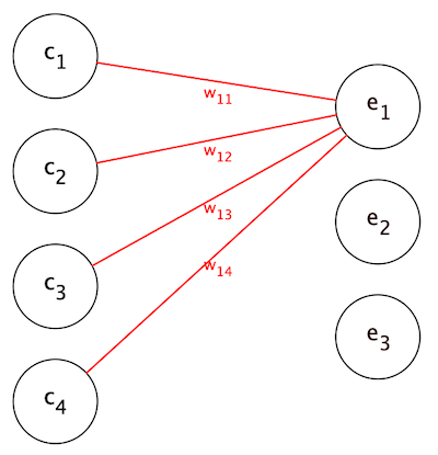
\(e_{1} = w_{11}c_{1} + w_{12}c_{2} + w_{13}c_{3} + w_{14}c_{4}\) is the weighted sum of the entries of the input vector \(\textbf{c}\). That is, each entry of the input vector \(\textbf{c}\) is scaled by a factor, and all the scaled entries are added together. The other entries \(e_{2}\) and \(e_{3}\) are also evaluated in the same way:
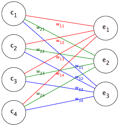
The fact that each entry of the output vector is a weighted sum of the entries of the input vector is an important property for us to exploit.
Suppose the absolute value of \(w_{11}\) is much greater than that of \(w_{12}\) (we consider absolute values because the weights can be negative). Then the term \(w_{11}c_{1}\) will have more influence on the weighted sum \(e_{1}\) than \(w_{12}c_{2}\). Recall that \(c_{1}\) and \(c_{2}\) represent the features sepal length and sepal width respectively. Setting the weight of each feature is essentially setting how influential each feature should be. In other words, we use these weights to extract information that is useful for performing the classification task.
Other than multiplying the weight matrix, we can also further transform the output vector by adding a constant vector to it. Let
\[\textbf{b} = \begin{pmatrix} b_{1}\\ b_{2}\\ b_{3} \end{pmatrix}\]Then, the matrix \(\textbf{Wc} + \textbf{b}\) will be
\[\begin{pmatrix} w_{11}c_{1} + w_{12}c_{2} + w_{13}c_{3} + w_{14}c_{4} + b_{1}\\ w_{21}c_{1} + w_{22}c_{2} + w_{23}c_{3} + w_{24}c_{4} + b_{2}\\ w_{31}c_{1} + w_{32}c_{2} + w_{33}c_{3} + w_{34}c_{4} + b_{3} \end{pmatrix}\]The matrix \(\textbf{b}\) just shifts each entry of \(\textbf{Wc}\) by a constant. Adding a vector to another one is also called translation. A combination of linear transformations and translations is called an affine transformation.
There are a few terminologies that you may encounter quite often. Let’s take a look of these terms.
- Artificial neural network (ANN): A machine learning model that utilizes affine transformations is called an artificial neural network.
Neural network
Despite the name contains 'neural network', and it is often said to be 'inspired' by how a human brain works, artificial neural network has very little to do with neuroscience.
- Neuron: An entry in the input or output vectors is called a neuron.
- Weight: The linear transformation matrix \(\textbf{W}\) above is called the weight matrix.
- Bias: The translation matrix \(\textbf{b}\) above is called the bias matrix.
- Parameter: The weights and biases are the parameters of the model.
Our first neural network
If you find that the above mathematics is a bit overwhelming, the good news is we don’t need to deal with the messy linear algebra when building an ANN with the TensorFlow Keras APIs. To begin, we import the TensorFlow library.
import tensorflow as tf
Then, we create a placeholder of the input vector.
inputs = tf.keras.Input(shape=(4, ))
Tensor
Actually, TensorFlow processes input vectors in batches. Therefore, thisInputdata structure is a multi-dimensional array called tensor (not to be confused with 'tensor' in various different mathematics contexts) instead of a single vector.
The parameter shape indicates that there are 4 entries in the input vector.
To create an affine transformation, we instantiate a Dense layer object.
affine_transformation = tf.keras.layers.Dense(units=3)
To apply the affine transformation to the input, we can call the Dense layer object with inputs as the parameter.
outputs = affine_transformation(inputs)
print(outputs)
Once executed, we can see that the output is a 3-dimensional vector.
To build a machine learning model with this affine transformation by instantiating a Model object.
model = tf.keras.Model(inputs=inputs, outputs=outputs)
model.summary()
For now, the weights and biases in our model are just random values. Therefore, this model can output garbage results only. We have an important question to ask: how do we know what these weights and biases should be? This is the ‘learning’ part of deep learning, and we are going to discuss this shortly. However, let’s explore the ‘deep’ part of deep learning first.
Deep neural network
In the previous section, we turned a higher dimensional feature vector into a lower dimensional output vector with the information that we need. Such affine transformation extracts useful information and discards useless information. However, what if the information of the feature vector is inadequate for extracting useful information?
Neural network provides a way to solve this problem. Recall that multiplying a \(n \times m\) matrix to a m-dimensional column vector will output a n-dimensional column vector. If \(n > m\), we should be able to produce a vector of higher dimension, i.e. the output vector has more information than the input vector!
Let say we want to transform the 4-dimensional feature vector of the Iris data set to a 6-dimensional vector, and use this 6-dimensional vector to produce the final result. In Keras, that means we need to use two Dense layers.
outputs_1 = tf.keras.layers.Dense(units=6)(inputs)
outputs_2 = tf.keras.layers.Dense(units=3)(outputs_1)
model = tf.keras.Model(inputs=inputs, outputs=outputs_2)
model.summary()
Theoretically, outputs_1 should contains more information than inputs as it has a higher dimension. The extra information may be useful for the model to produce better results in the final output.
However, there is a catch in this approach. Mathematically, the above code is equivalent to transforming the input vector \(\textbf{c}\) as follows:
\[\textbf{W}_{2}(\textbf{W}_{1}(\textbf{c})+\textbf{b}_{1}) + \textbf{b}_{2} = \textbf{W}_2\textbf{W}_{1}(\textbf{c}) + \textbf{W}_{2}(\textbf{b}_{1}) + \textbf{b}_{2}\]It is easy to verify that \(\textbf{W}_{2}\textbf{W}_{1}\) itself is a single \(4 \times 3\) matrix. Therefore, the input vector \(\textbf{c}\) is transformed directly to a 3-dimensional vector. The unhidden features are not really recovered.
This issue roots from the fact that the composite function of two linear functions is also just a linear function. Linear functions work well with data that are linearly distributed, but most data set are distributed in more complicated ways. We need a way to ‘disrupt’ the linearity of the composite function of the model. Activation functions are used for exactly this purpose.
Activation function
In deep learning, we put a non-linear activation function in between two affine transformations. The resulting composite function will no longer be a linear function and become a lot more flexible. With this technique, we can build a neural network model that can recover hidden information from the data by using multiple layers of affine transformations.
Neural networks with multiple layers of affine transformations are called deep neural networks, and this technique of machine learning is called deep learning.
The rectified linear unit (or ReLU) is a commonly used activation function. It basically sets all negative values to 0, i.e.
\[\begin{equation} \text{ReLU}(x) = \begin{cases} x & \text{if $x > 0$} \\ 0 & \text{if $x \leq 0$} \end{cases} \end{equation}\]We can apply the ReLU function to every entry of the output vector \(\textbf{Wc} + \textbf{b}\):
\[\begin{pmatrix} \text{ReLU}(w_{11}c_{1} + w_{12}c_{2} + w_{13}c_{3} + w_{14}c_{4} + b_{1})\\ \text{ReLU}(w_{21}c_{1} + w_{22}c_{2} + w_{23}c_{3} + w_{24}c_{4} + b_{2})\\ \text{ReLU}(w_{31}c_{1} + w_{32}c_{2} + w_{33}c_{3} + w_{34}c_{4} + b_{3}) \end{pmatrix}\]For simplicity, we denote this matrix by \(\text{ReLU}(\textbf{Wc} + \textbf{b})\). This composite function is no longer a linear function. When we stack multiple layers of these composite functions to form a model, this model will have very complicated behaviour. This enables deep neural networks to perform very complicated tasks.
In Keras, applying the activation function is simple. We only need to specify the activation parameter when creating the Dense layer. Let’s apply the ReLU function to the output of the first layer of affine transformation.
outputs_1 = tf.keras.layers.Dense(units=6, activation='relu')(inputs)
outputs_2 = tf.keras.layers.Dense(units=3)(outputs_1)
model = tf.keras.Model(inputs=inputs, outputs=outputs_2)
model.summary()
Softmax and sigmoid
Softmax and sigmoid are two other very commonly used activation functions.
And the softmax function is defined as
\[\sigma(z_i) = \frac{e^{z_{i}}}{\sum_{j=1}^K e^{z_{j}}} \ \ \ \text{for}\ i=1,2,\dots,K\]The definition looks a bit complicated. Let’s look at how softmax transforms some actual data.
test_input = np.array([[20, 30, 40, 50]], dtype='float')
test_tensor = tf.convert_to_tensor(test_input)
softmax = tf.keras.activations.softmax
test_softmax_output = softmax(test_tensor, axis=1)
print(f'Output of softmax: {test_softmax_output}')
print(f'Sum of softmax: {tf.reduce_sum(test_softmax_output, axis=1)}')
As we can see, softmax has the following properties:
- It outputs a number between 0 to 1.
- It preserves how big each entry of the array is, i.e. the bigger the value in the original array, the bigger the value that softmax will output.
- The sum of its outputs for all possible inputs is 1.
Therefore, softmax an ideal activation function for tasks involving the calculation of probabilities, such as the classification of Iris flower.
Let’s apply the softmax activation function to the final layer of our model.
outputs_1 = tf.keras.layers.Dense(units=6, activation='relu')(inputs)
outputs_2 = tf.keras.layers.Dense(units=3, activation='softmax')(outputs_1)
model = tf.keras.Model(inputs=inputs, outputs=outputs_2)
model.summary()
On the other hand, the sigmoid function is defined as
\[S(x) = \frac{1}{1+e^{-x}}\]When we perform binary classification (i.e. we only need to classify whether an item belongs to a class or not), the output vector can be of 1-dimensional as the probability of not belonging to the class can be found by \(1-p(\text{belongs to the class})\). In this case, the sigmoid activation function should be used instead of the softmax function.
Why do DNNs work?
At first, DNNs look like magic: they can be used to recover lost information out of nowhere! It seems that we don’t need to know what features we need at first to perform classification. Deep learning can recover or even discover the features for us.
However, this is not always the case. A neural network simply transforms a vector in a multistage manner. By representing the data in multiple forms (vectors of different dimensions), we may be able to extract the information we need.
From a machine learning perspective, deep learning is not too different from finding best-fit lines. The only difference is rather than using a single straight line, we fit a curve in a higher dimensional latent space to the data. We still assume that the data change in this latent space in a predictable manner. We also train the model so that the curve is a good representation of how the data change. Finally, we use the curve to make predictions with unseen data.
Therefore, there is no other thing that can replace a representative and clean data set. If the data set is a good sample of the population, it will be more likely for us to train a deep learning model that can fit the latent space of the population and make better predictions.
Train the neural network
Loss functions
For now, the parameters in our model are just some random numbers. This model cannot do any meaningful predictions. So what should be these weights and biases? However, we need to ask another important question first: how bad is this model? We need an objective indicator to determine this.
Let’s look at the setosa datum [5.1, 3.5, 1.4, 0.2] once again. After one-hot encoding, the label setosa is represented by [1, 0, 0].
Suppose our randomly initialised neural network outputs [0.1, 0.2, 0.7] when [5.1, 3.5, 1.4, 0.2] is inputted to the model. The vectors [1, 0, 0] and [0.1, 0.2, 0.7] can be considered as two points in the 3-dimensional space. Recall that the distance between two points can be found by the distance formula:
If the output of our neural network is closer to the real answer, the ‘distance’ between the output vector and answer vector will be smaller. Thus, this ‘distance’ can be used to measure how much error the model has made. We call this measurement of error a loss function.
In practice, we use different loss functions for different purposes. For example, classification tasks typically use cross entropy as the loss function. This loss function is a bit more complicated, but using it in Keras is very simple. We can set the loss function by calling the compile method of the model:
model.compile(loss='categorical_crossentropy')
The smaller the loss function, the better the model performs. Therefore, our goal of adjusting the parameters of the model is to minimise the loss function. The technique to reduce the loss is gradient descent.
Gradient descent
Our model has many parameters so it is quite hard to imagine what strategy we should use to change the parameters in order to minimise the loss function. Let’s look at a much simpler function: a loss function \(L(w)\) which takes a single parameter \(w\). The function looks like this:
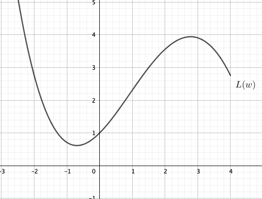
Suppose the current value of the parameter \(w\) is 2. We can find the value of the loss function from the graph:
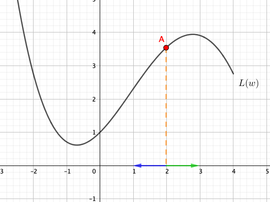
In order to minimise the value of the loss, how should \(w\) be changed? Should the point \(A\) move to the left or the right? From the graph, we can see that it should move to the left.
But what if the current value of \(w\) is -2?
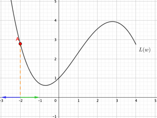
We can see that it should move to the right now. Can you observe the pattern?
Consider the slope of the graph at point \(A\). When \(w=2\), the slope at point \(A\) is positive. We can easily see that whenever the slope is positive, we can decrease the value of \(w\) to reduce the value of \(L\).
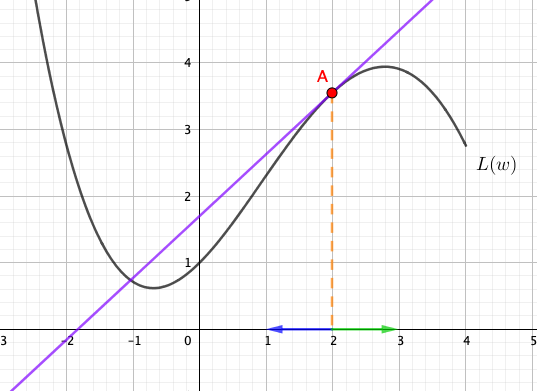
Similarly, whenever the slope is negative, we can increase the value of \(w\) to reduce the value of \(L\).
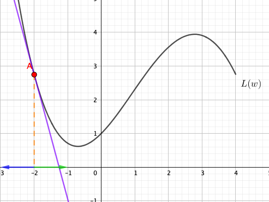
Mathematically, the slope of the curve at \(w=w_{0}\) is \(L'(w_{0})\), where \(L'\) is the derivative of the function \(L\). Notice that:
- The sign of the change in \(w\) at \(w=w_{0}\) is opposite to the slope at that point.
- The absolute value of the slope is bigger (i.e. the tangent is steeper) when \(A\) is away from the minimum position.
Therefore, in order to reduce the value of \(L\), the amount of the parameter \(w\) changes, \(\Delta w\), should:
- have its sign opposite to the derivative,
- have its absolute value proportional to the absolute value of the derivative.
Therefore, we can define
\[\Delta w = -L'(w_{0})\]In practice, we may not want to change the value of \(w\) by a full derivative of that point. Otherwise, the point \(A\) may overshoot the minimum location, and it may never settle in at the minimum position. Therefore, we often multiply the negative derivative by a small factor \(\lambda\) called the learning rate:
\[\Delta w = -\lambda L'(w_{0})\]Our model has many more parameters, but the same principle can be used to update the parameters. For a loss function \(G\) and a collection of parameters \(W\), the gradient vector \(\nabla G\) at a multidimensional point \(W_{0}\) is evaluated. The gradient vector can be considered as a generalisation of slope in a higher dimensional space. It always points to the direction of greatest increase. Therefore, the negative of \(\nabla G(W_{0})\) always points to the direction of greatest decrease. Hence, the changes in the parameters at a learning rate \(\gamma\) can be defined as
\[\Delta W = -\gamma \nabla G(v_{0})\]This gradient-based method of updating the model’s parameters is called gradient descent. There are a few gradient descent algorithms. The simplest mini-batch stochastic gradient descent works as follows:
- Draw a batch of samples \(\textbf{x}\) and the corresponding targets \(\textbf{y}_\text{true}\).
- Apply the model on \(\textbf{x}\) and obtain the predictions \(\textbf{y}_\text{pred}\).
- Calculate the mismatch between \(\textbf{y}_\text{true}\) and \(\textbf{y}_\text{pred}\) with a loss function.
- Compute the gradients of the loss function with respect to the parameters of the model.
- Update the parameters of the model by moving the parameters slightly in the opposite direction of the gradient vector.
Fortunately, we don’t need to deal with this complexity in Keras to train the neural network. All we need to do is to specify the optimizer when calling the compile method of the model.
model.compile(optimizer='sgd', loss='categorical_crossentropy')
Our model is finished. All we need to do is to feed the training data into it and train it. Let’s prepare some training data.
Dividing a data set
We should always divide the data set into the training and testing data sets first. We need a testing data set that is not seen by the model to test the model accurately.
# Separate the data set into the training data set and testing data set
# Create a list of indices
indices = np.arange(len(features))
# Shuffle the list of indices
np.random.shuffle(indices)
# We use 80% of the data for the training
bound = int(0.8 * len(indices))
# Split the data sets by slicing the NumPy arrays
x_train, x_test = features[indices[:bound]], features[indices[bound:]]
y_train, y_test = vectorized_labels[indices[:bound]], vectorized_labels[indices[bound:]]
To train the model, we just need to call the fit method with the training data.
model.fit(x_train, y_train,epochs=500, validation_data=(x_test, y_test))
The parameter epochs specifies how many times the training data set is fed to the model for training.
After the training, we can get a datum and test whether the model works:
test_index = bound + 1
result = model.predict(features[test_index:test_index+1])
print(f'Predicted: {class_names[np.argmax(result)]}')
print(f'Real: {class_names[labels[test_index]]}')
Summary
- Vector is a fundamental data structure for deep learning. A vector is an array of values. We can use vectors to represent different information.
- An affine transformation can transform a vector into another vector. The dimension of the input vector can be smaller or bigger than the dimension of the output vector, depending on what the affine transformation is.
- Deep learning is a machine learning method that utilises multiple layers of affine transformations to transform feature vectors into vectors with information that we want.
- The weights and biases of the affine transformations in a deep learning model are the parameters of the models. The values of these parameters are determined during the training process.
- Activation functions make deep learning models more capable of dealing with complicated tasks. Common activation functions include ReLU, softmax and sigmoid.
- The softmax activation function is suitable for the output layer of a classification model.
- We need to define a loss function for the training process to measure how much error the model makes.
- We use gradient descent to update the parameters of a deep learning model. The training data are fed to the model, and loss function is evaluated. The gradients of the loss function with respect to the parameters are computed. The parameters are updated by moving to the opposite direction of the gradient vector.